# 하드웨어 인식 동적 추측 디코딩(DSD): 배치 크기에 맞춰 초안 토큰 수를 조절하는 추론 최적화 (feat. Cohere)
**URL:** https://discuss.pytorch.kr/t/dsd-feat-cohere/11200
**Category:** 읽을거리&정보공유
**Tags:** inference, vllm, gpu, cohere, moe, llm, speculative-decoding
**Created:** [7월 12, 2026, 1:30오전 UTC](https://discuss.pytorch.kr/t/dsd-feat-cohere/11200 "2026-07-12T01:30:55Z")
**Posts on this page:** 1
**Page:** 1
### Author:  [@9bow](https://discuss.pytorch.kr/u/9bow)
#### Post date: [7월 12, 2026, 1:30오전 UTC](https://discuss.pytorch.kr/t/dsd-feat-cohere/11200/1 "2026-07-12T01:30:55Z")
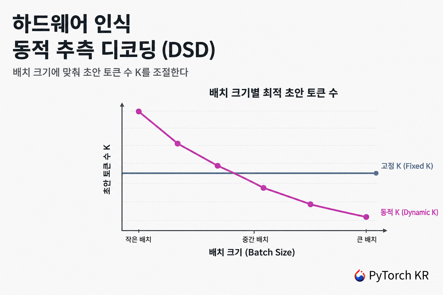
## 하드웨어 인식 동적 추측 디코딩(DSD) 소개
대규모 언어 모델(LLM)은 한 번에 토큰 하나씩 생성합니다. 이 순차적 특성 때문에 실제 서비스에서 체감하는 속도는 GPU의 연산 능력이 아니라 "다음 토큰 하나를 얼마나 빨리 뽑아내느냐"에 크게 좌우됩니다. 이 병목을 완화하는 대표적인 기법이 **추측 디코딩(Speculative Decoding, SD)** 입니다. 작고 빠른 _초안(draft) 모델_ 이 여러 토큰을 미리 제안하면, 크고 정확한 _타겟(target) 모델_ 이 그 토큰들을 한 번의 타임스텝에 한꺼번에 검증합니다. 한 스텝에 여러 토큰이 받아들여질 수 있으므로, 출력 품질을 전혀 손상하지 않으면서 생성 속도를 끌어올립니다.
그런데 이 추측 디코딩에는 오래된 약점이 하나 있습니다. 실제 프로덕션 환경에서는 여러 요청을 묶어 처리하는 **배칭(Batching)** 이 필수인데, 배치 크기(Batch Size, BS)가 커지면 추측 디코딩의 이점이 사라지고 오히려 _느려지기도_ 합니다. 초안 모델이 몇 개의 토큰(K개)을 미리 뽑을지 정하는 값 K를 고정해 두면, 어떤 상황에서는 도움이 되지만 다른 상황에서는 손해를 보는 셈입니다. [Cohere](https://cohere.com/)가 공개한 **하드웨어 인식 동적 추측 디코딩(Hardware-Aware Dynamic Speculative Decoding, DSD)** 은 바로 이 문제를 정면으로 다룹니다. 핵심 아이디어는 단순하면서도 강력합니다. _K를 고정하지 말고, 모델과 하드웨어의 상호작용에 맞춰 매 순간 최적의 K를 동적으로 고르자_ 는 것입니다.
이 글에서는 추측 디코딩이 GPU의 어떤 특성을 이용해 속도를 얻는지부터, 왜 배치 크기가 커지면 그 이점이 무너지는지, 그리고 DSD가 어떻게 최적의 K를 찾아내는지를 차례로 살펴봅니다. 나아가 Cohere가 이 최적화를 실제 프로덕션급 추론 엔진인 [vLLM](https://github.com/vllm-project/vllm)에 기여하면서 마주한 엔지니어링 난관 — 비동기 스케줄링(Async Scheduling)과 Full CUDA Graph 같은 고급 최적화와의 호환성 — 까지 다룹니다. 단순한 아이디어가 고도로 최적화된 실제 시스템 안에 자리 잡기까지 무엇이 필요했는지를 함께 짚어보는 것이 이 글의 목표입니다.
## 추측 디코딩의 원리: 유휴 연산 자원을 활용하는 트레이드오프
추측 디코딩이 어떻게 속도를 얻는지 이해하려면, 먼저 GPU 추론이 두 가지 서로 다른 병목에 걸린다는 사실을 알아야 합니다. GPU 추론의 비용은 **연산(compute)** 과 **메모리 대역폭(memory bandwidth)** 사이의 트레이드오프로 결정되며, 어느 쪽이 병목이 되는지는 배치 크기에 달려 있습니다.
- **작은 배치 크기(small BS)** 에서는 추론이 **메모리 대역폭 병목(memory bandwidth-bound)** 상태입니다. LLM의 가중치를 HBM(고대역폭 메모리)에서 SRAM으로 불러오는 비용이 지배적이기 때문입니다.
- **큰 배치 크기(large BS)** 에서는 추론이 **연산 병목(compute-bound)** 상태로 바뀝니다. 많은 요청 토큰에 대해 LLM 가중치를 곱하는 행렬 연산이 지배적이 되기 때문입니다.
추측 디코딩에 걸리는 시간은 크게 두 부분으로 나뉩니다.
\text{추측 디코딩 시간} = \text{초안 토큰 생성 시간(작은 초안 모델)} + \text{초안 토큰 검증 시간(큰 타겟 모델)}
초안 모델은 실행 비용이 훨씬 저렴합니다. 초안이 K개의 토큰을 만들면 타겟 모델은 \text{BS} \times (K+1) 개의 토큰을 처리해야 하는데, 같은 배치 크기 기준으로 K+1 배 더 많은 연산을 하게 되므로 **검증(verify)** 이 병목이 됩니다. 여기서 추측 디코딩의 묘수가 드러납니다. 현대 GPU에서 연산 장치는 메모리 대역폭보다 대략 두 자릿수(약 100배) 빠릅니다. 그래서 작은 배치 크기의 메모리 대역폭 병목 구간에서는 연산 장치가 대부분 놀고 있습니다. 추측 디코딩은 바로 이 놀고 있는 연산 자원을 활용해, 검증 단계에서 K+1 배 많은 토큰을 타겟 모델에 밀어 넣습니다. 어차피 낭비되고 있던 연산을 공짜로 활용하는 셈입니다.
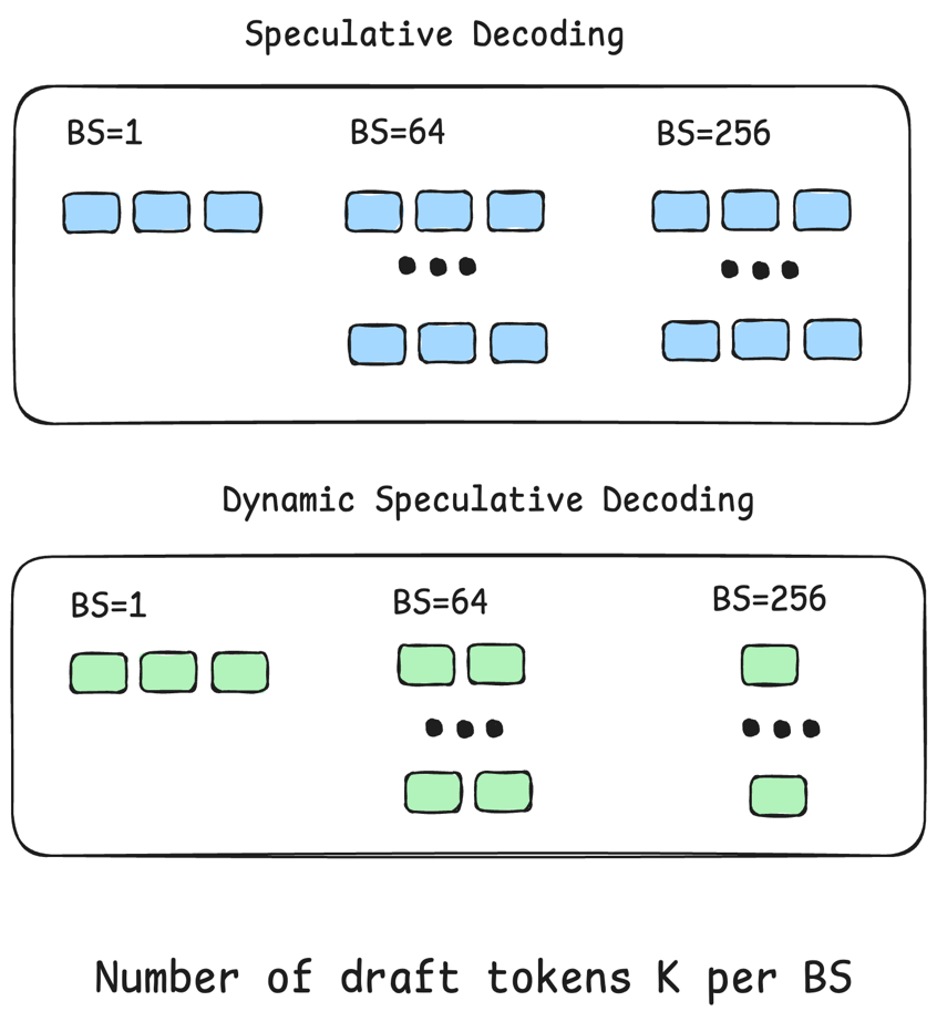
위 그림은 이 글의 핵심을 한눈에 보여줍니다. 위쪽의 기존 추측 디코딩은 BS=1이든 BS=64든 BS=256이든 항상 같은 개수의 초안 토큰(파란 블록)을 뽑습니다. 반면 아래쪽의 동적 추측 디코딩(초록 블록)은 배치 크기가 커질수록 초안 토큰 수를 줄입니다. 왜 이렇게 해야 하는지는 다음 절에서 살펴봅니다.
### 왜 배치 크기가 커지면 추측 디코딩이 무너지는가
문제는 배치 크기가 커질 때 발생합니다. 배치 크기가 커지면 일반적인 LLM 추론은 점점 더 연산 병목 상태가 되고, 결국 추측 디코딩이 활용할 유휴 연산이 남지 않습니다. 이 구간에서는 검증에 드는 추가 연산이 고스란히 부담으로 돌아와, 추측 디코딩이 일반 추론보다 오히려 _더 느려질_ 수 있습니다. 그런데 프로덕션 시스템에서 배치 크기는 좀처럼 작지 않고, 트래픽에 따라 시시각각 변합니다. 고정된 K를 쓰는 추측 디코딩이 실제 서비스에서 널리 쓰이지 못하는 이유가 여기에 있습니다.
## 프로덕션과 강화학습이 요구하는 것: 하드웨어에 맞춘 K
배치 크기 문제 외에도, 추측 디코딩의 개선을 강하게 요구하는 또 다른 무대가 있습니다. 바로 **강화학습(Reinforcement Learning, RL)** 입니다.
강화학습은 모델 가중치를 갱신하는 **학습(training)** 단계와, 학습에 쓸 데이터 및 보상 신호를 만들어 내는 **롤아웃(rollout)** 단계를 번갈아 수행합니다. 이 중 롤아웃 단계가 주된 병목으로, [전체 자원의 최대 85%](https://microsoft.ai/pdf/mai-thinking-1.pdf)까지 소비할 수 있습니다. 강화학습을 키우는 것이 모델 지능을 끌어올리는 중요한 축인 만큼, 롤아웃 추론을 가속하는 일은 반드시 풀어야 할 문제입니다.
그러나 추론 모델(reasoning model)을 쓰는 강화학습은 **롱테일(long-tail) 분포** 를 만들어 냅니다. 배치 안의 요청 하나가 유독 오랫동안 생성을 이어가면서 나머지 배치 전체를 붙잡아 두고 자원을 낭비시키는 것입니다. 추측 디코딩은 바로 이런 롱테일 생성을 가속하는 데 도움이 되지만, 앞서 본 것처럼 높은 배치 크기에서 처리량(throughput)을 떨어뜨리기 때문에 전체 배포 환경에서의 실용성이 제한됩니다.
동적 배칭과 강화학습, 이 두 난관은 결국 같은 요구로 수렴합니다. _더 나은 추측 디코딩 시스템은 하드웨어 제약에 따라 최적의 K를 제어할 수 있어야 한다_ 는 것입니다. 그래야 완전한 프로덕션 시스템과 대규모 강화학습 롤아웃에서 모두 유용하게 쓸 수 있습니다.
## 동적 추측 디코딩(DSD)의 핵심 아이디어
여기서 하드웨어 인식 동적 추측 디코딩(DSD)이 등장합니다. DSD는 초안 토큰의 개수를 상황에 맞게 조절함으로써 기존 추측 디코딩을 개선합니다. 기존 추측 디코딩에서 K는 고정값이지만, DSD에서는 모델과 하드웨어 사이의 상호작용을 근거로 최적의 K를 선택합니다. 구체적으로, DSD는 추론이 메모리 대역폭 병목일 때 K를 늘리고, 연산 병목일 때 K를 줄입니다.
이 규칙이 모델 구조에 따라 어떻게 다르게 나타나는지가 흥미롭습니다.
**밀집(Dense) 모델** 의 경우, 일반적으로 낮은 배치 크기에서 높은 K를, 높은 배치 크기에서 낮은 K를 씁니다. 즉 배치 크기가 커질수록 최적 K는 **단조 감소(monotonically decreasing)** 합니다.
**전문가 혼합(Mixture-of-Experts, MoE) 모델** 의 경우, 최적 K는 배치 크기에 대해 **비단조(non-monotonic)** 로 움직입니다. 이유는 다음과 같습니다.
- **낮은 배치 크기** 에서는 검증이 추가 전문가(expert)를 불러와야 하므로 최적 K가 낮게 시작합니다.
- **중간 배치 크기** 에서는 이미 거의 모든 전문가가 메모리에 올라와 있어서, 검증이 추가로 불러올 전문가가 거의 없습니다. 그래서 최적 K가 오히려 커집니다.
- **높은 배치 크기** 에서는 밀집 모델과 마찬가지로 연산 병목이 되므로 최적 K가 다시 작아집니다.
MoE와 추측 디코딩의 상호작용에 대한 더 깊은 논의는 Cohere가 앞서 발행한 [MoE 모델과 추측 디코딩에 관한 블로그](https://cohere.com/blog/mixture-of-experts-models-get-more-from-speculative-decoding)에서 확인할 수 있습니다.
### 최적의 K를 찾는 지표: goodput
그렇다면 최적의 초안 토큰 개수는 어떻게 찾을까요? 핵심은 K에서 K+1로 초안 토큰을 하나 더 늘렸을 때의 _한계 기여(marginal contribution)_ 를 이해하는 것입니다. 초안 토큰 하나를 처리하는 **연산 비용은 위치와 무관하게 동일** 합니다. 첫 번째 초안 토큰이든 마지막 초안 토큰이든 처리 비용은 같습니다. 그러나 그 토큰이 **수용 길이(Acceptance Length, AL)** 에 기여하는 정도는 위치에 크게 좌우됩니다. 수용 확률은 위치에 따라 [지수적으로 감소](https://proceedings.mlr.press/v202/leviathan23a/leviathan23a.pdf)하므로, 앞쪽 토큰이 뒤쪽 토큰보다 훨씬 더 높은 확률로 받아들여집니다. 따라서 초안 토큰을 하나 더 추가할 때의 이 트레이드오프를 담아내는 지표가 필요합니다.
[TurboSpec](https://arxiv.org/abs/2406.14066) 같은 기존 DSD 연구는 이 지표로 **goodput** 을 사용합니다. Cohere 역시 goodput을 쓰되, 다음과 같이 단순화했습니다.
\text{goodput} = \frac{\text{AL}}{\text{ITL}}
여기서 AL은 수용 길이(Acceptance Length), ITL은 **토큰 간 지연(Inter-Token Latency)** 으로 대체로 초안 생성 시간과 검증 시간의 합입니다. 이 지표는 K개의 초안 토큰이 AL에 기여하는 한계 효과와, 그에 드는 실제 벽시계 시간(wall clock cost) 사이의 트레이드오프를 포착합니다. 값이 클수록 더 좋은 가속을 의미합니다. 이렇게 단순하게 정의하면 DSD를 미래의 다양한 모델 아키텍처에 적용하기 쉬워지고, ITL이 이미 모든 연산의 종합적 영향을 담고 있으므로 각 구성 요소를 개별적으로 프로파일링한 뒤 다시 조합할 필요가 없습니다.
실제 동작 방식은 이렇습니다. 오프라인 프로파일링으로 AL과 ITL을 측정해 최적의 K를 찾고, 이를 **룩업 테이블(lookup table)** 로 저장해 런타임에 사용합니다. 이 오프라인 테이블은 콜드 스타트(cold-start) 문제를 해결하며, 확장성도 갖춥니다. 엔진의 런타임 지표에서 얻는 실시간 AL과 ITL 통계를 반영할 수 있어, 변화하는 워크로드에 맞춰 DSD가 적응하도록 만들 수 있습니다.
## 실험 결과: Dense와 MoE에서 최적 K는 어떻게 달라지는가
Cohere는 세 가지 구성을 비교했습니다. 추측 디코딩을 쓰지 않는 **바닐라(vanilla)**, 고정 K 추측 디코딩( **fixed-K SD** , [EAGLE](https://arxiv.org/abs/2401.15077) 초안 헤드를 K=3으로 고정한 기준선), 그리고 동적 K를 쓰는 **DSD** 입니다. 데이터셋은 [MT-Bench](https://arxiv.org/abs/2306.05685)를 사용했고, 샘플 수를 20 \times \text{BS} 로 업샘플링해 배치 크기당 20번의 웨이브(wave)가 사용되도록 했습니다.
먼저 DSD가 선택한 최적 K를 밀집 모델인 [Command A](https://discuss.pytorch.kr/t/command-a-cohere/6611)와 MoE 모델인 [Command A+](https://discuss.pytorch.kr/t/cohere-command-a-moe/10321)에 대해 각각 프로파일링했습니다. 실측 결과는 앞서 설명한 경향을 그대로 검증합니다. 밀집 모델에서는 배치 크기가 커질수록 최적 K가 단조 감소하는 반면, MoE 모델에서는 그렇지 않았습니다. Command A+ 는 중간 배치 크기 구간에서 더 높은 최적 K에 도달할 수 있었습니다.
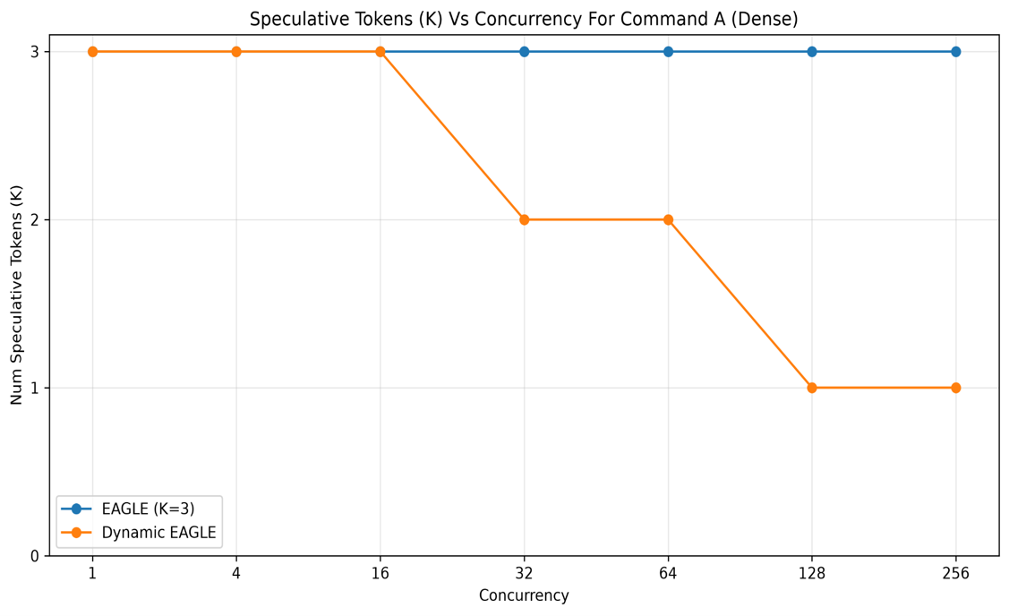
밀집 모델인 Command A의 그래프를 보면, 고정 K(파란 선, EAGLE K=3)는 배치 크기와 무관하게 항상 3으로 유지되는 반면, 동적 K(주황 선, Dynamic EAGLE)는 동시성 16까지 3을 유지하다가 32에서 2로, 128부터는 1로 단조 감소합니다.
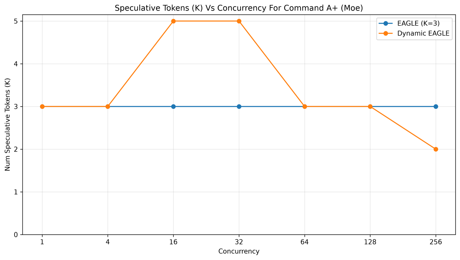
반면 MoE 모델인 Command A+ 의 그래프는 뚜렷하게 다른 모양을 그립니다. 동적 K는 동시성 16과 32 구간에서 5까지 치솟았다가, 그 전후로는 3, 그리고 아주 높은 배치 크기(256)에서 2로 떨어집니다. 산봉우리 모양의 이 곡선이 바로 MoE 특유의 비단조성을 보여줍니다.
### TOPS/user로 본 실제 속도 향상
Cohere는 사용자당 초당 출력 토큰 수인 **TOPS/user(Token Output Per Second, per user)** 로 실제 속도를 측정했습니다. 밀집 모델 Command A에서 DSD의 이점은 배치 크기 전 구간에 걸쳐 분명합니다.
- **낮은 배치 크기** 에서 DSD는 SD(K=3)와 동일한 가속을 냅니다.
- **높은 배치 크기(64/128)** 에서 DSD는 SD와 바닐라 모두보다 빠릅니다.
- **아주 높은 배치 크기(256)** 에서 DSD는 바닐라의 TOPS와 대등한데, 이 구간에서 SD는 BS 128과 256에서 오히려 성능이 퇴보(regress)합니다.
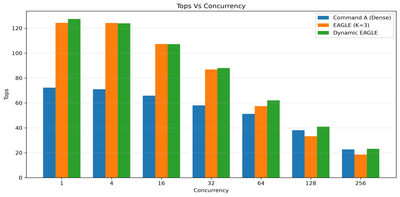
구체적인 수치로 보면, DSD는 BS 128과 BS 256 모두에서 **SD보다 약 23% 빠릅니다**. 또한 **BS 128에서 바닐라보다 7.5% 빠르고** , **BS 256에서 1.82% 빠릅니다**. 반면 SD는 이 구간에서 바닐라 대비 성능이 퇴보합니다. 다시 말해 DSD는 추측 디코딩이 도움이 되는 구간에서는 그 가속을 그대로 취하고, 고정 K SD라면 오히려 손해를 볼 구간에서는 바닐라 성능 쪽으로 우아하게 되돌아갑니다(gracefully falls back).
MoE 모델 Command A+ 에서는 SD와 DSD가 비슷한 가속을 보였습니다. DSD가 배치 크기 대부분의 구간에서 K=3을 선택해 고정 K SD와 같아졌기 때문인데, BS 16에서 32 사이에서만 K=5를 골랐습니다. 다만 이 더 높은 K는 추가 가속으로 이어지지 못했습니다. 그 이유는 EAGLE 헤드가 단일 타임스텝을 위해 학습되었는데 K \> 1인 여러 타임스텝에 재사용되다 보니, 수용률이 충분히 높지 않아 이득이 나지 않았기 때문으로 보입니다. Cohere는 [EAGLE-3](https://arxiv.org/abs/2503.01840)나 [DFlash](https://arxiv.org/abs/2602.06036) 같은 더 최신 기법이라면 이 시나리오에서 더 뚜렷한 이득을 보일 것으로 기대합니다.
## vLLM에 기여하기: 고도로 최적화된 프레임워크와의 호환성
DSD의 진짜 도전은 아이디어 자체가 아니라, 이를 [vLLM](https://github.com/vllm-project/vllm)처럼 고도로 최적화된 추론 프레임워크 안에서 구현하는 데 있었습니다. Cohere는 올해 초 이 최적화를 vLLM에 기여했습니다([Pull Request](https://github.com/vllm-project/vllm/pull/32374), 사용법은 [vLLM 문서](https://docs.vllm.ai/en/latest/features/speculative_decoding/dynamic_speculative_decoding/) 참고). DSD라는 개념 자체는 새롭지 않고 단순 구현이라면 간단하지만, 문제는 vLLM이 탑재한 수많은 최적화와 모두 호환되어야 한다는 것이었습니다. vLLM은 **비동기 스케줄링(async scheduling)** 이나 **Full CUDA Graph** 같은 최적화를 제공하는데, DSD가 vLLM의 효율을 온전히 끌어내려면 이들과 전부 어우러져야 합니다. 아래에서 가장 중요한 두 가지를 살펴봅니다.
### 비동기 스케줄링(Async Scheduling)과의 호환
추론 프레임워크는 먼저 요청을 **스케줄링(scheduling)** 하고(CPU 작업), 그다음 모델 추론(model inference)을 실행합니다(GPU 작업). 역사적으로는 GPU가 병목이었지만, 프로덕션급 GPU가 빨라지면서 상대적으로 CPU 스케줄링 오버헤드가 커졌습니다. GPU가 일을 일찍 끝내고 다음 배치가 스케줄링되기를 기다리게 된 것입니다. 이를 해결하기 위해 vLLM은 [**비동기 스케줄링**](https://vllm.ai/blog/2026-03-24-mrv2)을 도입했습니다. 타임스텝 T+1의 스케줄러(CPU)를 타임스텝 T의 모델 러너(GPU)와 겹쳐 실행함으로써, 스케줄러 지연을 감추는 방식입니다.
여기서 핵심은, T+1의 스케줄러가 아직 병렬로 실행 중인 T의 모델 러너 출력 _없이_ 동작한다는 점입니다. 이것이 가능한 이유는 스케줄러가 CPU에서 한 스텝 앞서, 순수하게 개수(count)와 자리표시자(placeholder)만으로 동작하기 때문입니다. 실제 토큰 값은 GPU에 존재하며, 한 스텝 뒤에 모델 러너가 GPU 측 스캐터(scatter)를 통해 소비합니다. 프로세스 경계를 넘나드는 것은 자리표시자와 토큰 개수 같은 가벼운 카운트뿐이며, 이마저도 비동기로 오갑니다.
스케줄러는 모델 러너에게 이번에 초안 토큰을 몇 개 생성할지, 그리고 이전 타임스텝의 초안 토큰 중 몇 개를 이번에 검증할지를 알려줍니다. 그런데 DSD는 _매 타임스텝마다 같은 개수의 초안 토큰이 생성되고 검증된다_ 는 기존 가정을 깨뜨립니다. 이 때문에 스케줄러와 모델 러너 양쪽의 장부 관리(bookkeeping)가 달라집니다.
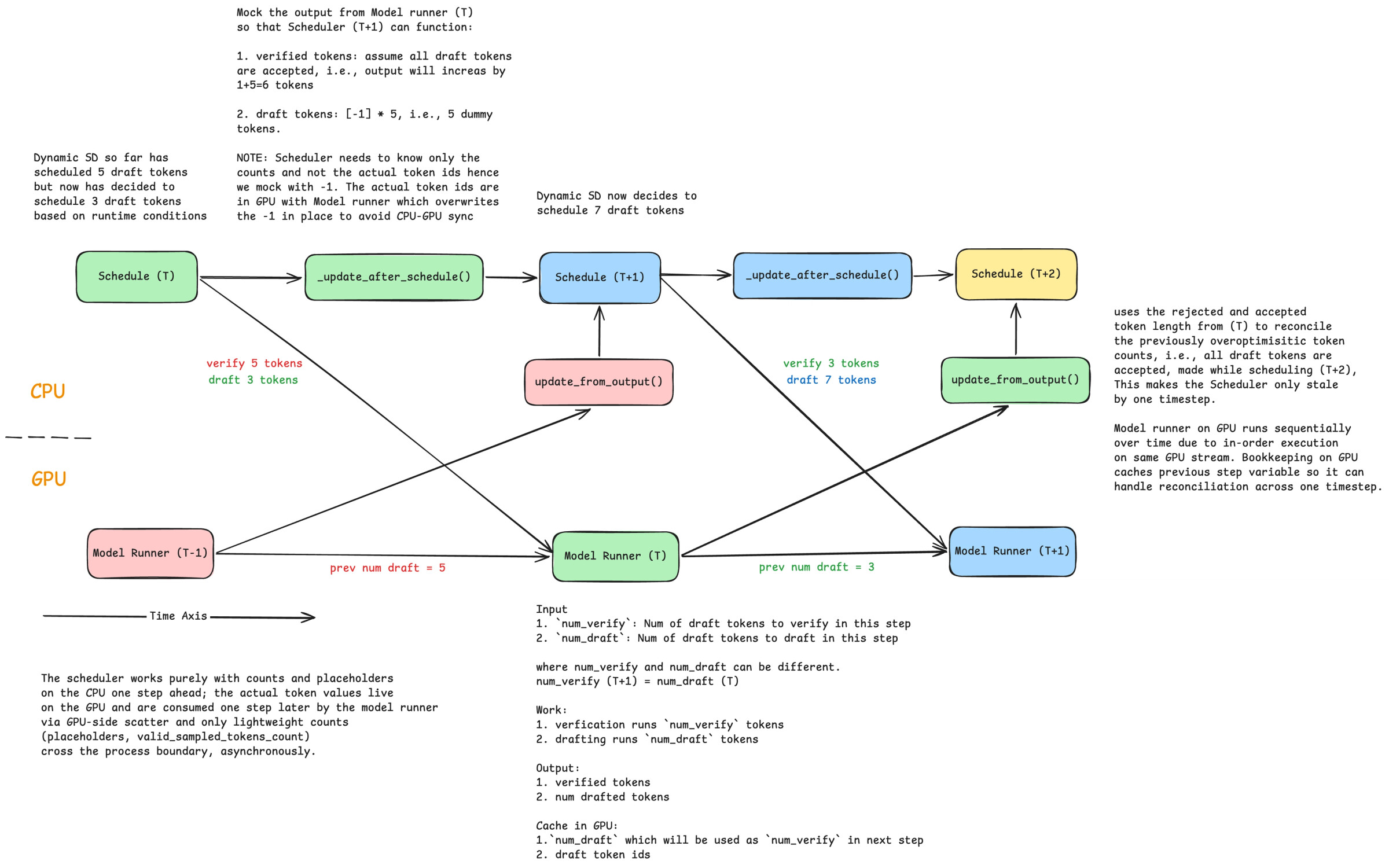
위 다이어그램은 비동기 스케줄링 아래에서 DSD가 여러 타임스텝에 걸쳐 어떻게 동작하는지를 보여줍니다(자세히 보려면 확대). 이 예시에서 시스템은 T-1까지 5개의 토큰을 초안으로 만들다가, T에서 3개로, 그리고 T+1에서 7개로 바꿉니다. 스케줄러는 실제 토큰 ID가 아니라 개수만 알면 되므로 더미 값 -1로 자리를 채워 두고(mock), 실제 토큰 ID는 GPU의 모델 러너가 CPU-GPU 동기화를 피하기 위해 그 자리에서 덮어씁니다. `num_verify` (이번 스텝에 검증할 초안 토큰 수)와 `num_draft` (이번 스텝에 초안으로 만들 토큰 수)가 서로 다를 수 있으며, 관계는 `num_verify(T+1) = num_draft(T)` 로 이어집니다.
### Full CUDA Graph와의 호환
모델의 순전파(forward pass)는 수많은 CUDA 커널(kernel)을 실행하는데, 커널을 하나 실행할 때마다 CPU 오버헤드가 발생합니다. 현대의 프로덕션급 GPU가 빨라질수록, 수많은 커널에 걸쳐 누적되는 이 실행 오버헤드가 전체 추론 시간에서 무시할 수 없는 비중을 차지하게 됩니다. **Full CUDA Graph(FCG)** 는 워밍업(warmup) 단계에서 모든 커널 실행을 한 번 캡처해 두었다가, 이를 개별 실행이 아니라 하나의 그래프 실행으로 재생(replay)함으로써 이 오버헤드를 제거합니다.
vLLM은 디코드(decode) 요청에 대해 `<배치 내 토큰 수, 고정 K>` 튜플을 캡처하는 방식으로 [FCG를 지원](https://docs.vllm.ai/en/latest/design/cuda_graphs/)합니다. DSD는 이를 `<배치 내 토큰 수, 서로 다른 최적 K>` 로 확장해 더 많은 조합을 기록함으로써, 런타임에 K가 바뀌어도 여전히 캡처된 CUDA 그래프에 적중하도록 만듭니다([Pull Request](https://github.com/vllm-project/vllm/pull/45953)).
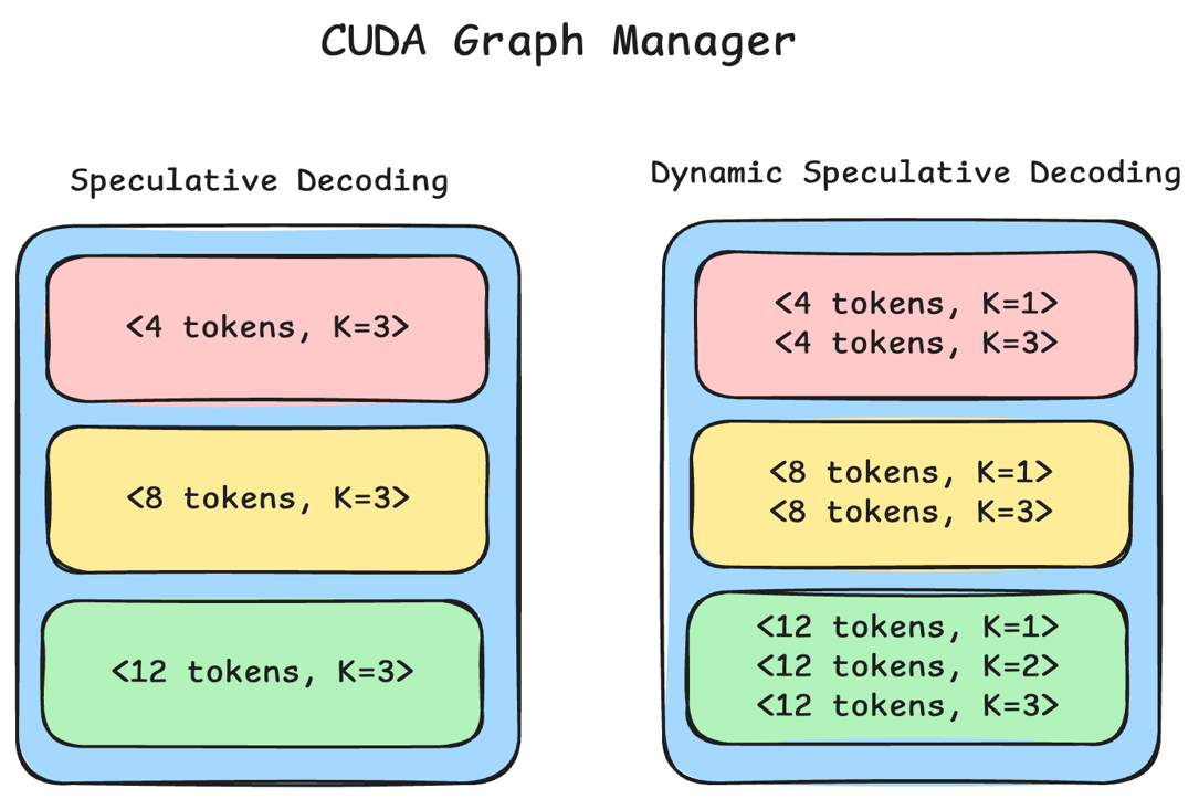
위 그림은 최대 K=3인 예시를 보여줍니다. 배치에 토큰이 8개 있을 때, 기존 SD는 `<8 tokens, K=3>` 하나만 캡처합니다. 반면 DSD는 토큰 수가 K+1로 나누어떨어지는 모든 유효한 K를 캡처합니다. 즉 `<8 tokens, K=1>` 과 `<8 tokens, K=3>` 을 모두 기록합니다. 토큰 수가 K+1로 나누어떨어진다는 것은 배치 안의 모든 요청이 디코드 요청이라는 뜻이며, 이것이 바로 vLLM에서 FCG로 라우팅되는 조건입니다.
## 결론: 단순한 지표 하나로 실용성을 되찾다
DSD가 보여준 것은, 추측 디코딩이라는 오래된 기법을 실제 프로덕션에서 쓸모 있게 만드는 열쇠가 화려한 새 알고리즘이 아니라 _하드웨어 상태에 맞춰 K를 조절하는 단순한 goodput 지표_ 였다는 사실입니다. 밀집 모델에서 DSD는 SD가 손해를 보던 높은 배치 크기 구간에서 SD 대비 약 23%의 속도 향상을 되찾으면서, 추측 디코딩이 무익하거나 해로운 구간에서는 바닐라 성능으로 안전하게 후퇴합니다. 이는 배치 크기가 시시각각 변하는 실제 서비스와, 롱테일 생성이 자원을 붙잡는 대규모 강화학습 롤아웃 모두에서 추측 디코딩을 비로소 실전에 투입할 수 있게 해줍니다.
동시에 이 작업은 좋은 아이디어를 실제 시스템에 녹여 내는 일이 얼마나 까다로운지도 잘 보여줍니다. 비동기 스케줄링과 Full CUDA Graph처럼 이미 고도로 최적화된 구성 요소들의 가정을 하나씩 다시 맞춰 나가야 했고, 그 과정이 vLLM 커뮤니티와의 협업으로 이뤄졌습니다. Cohere는 특히 [Red Hat](https://www.redhat.com/)의 Lucas Wilkinson과 [NVIDIA](https://www.nvidia.com/)의 Benjamin Chislett이 vLLM PR을 함께 논의하고 리뷰해 준 데 특별한 감사를 전했습니다. MoE 모델에서 아직 기대만큼의 이득이 나오지 않은 점은, EAGLE 헤드를 여러 타임스텝에 재사용하는 데서 오는 한계로 지목되었으며, EAGLE-3나 DFlash 같은 후속 기법으로 개선될 여지를 남겨 두었습니다. 추론 효율을 다루는 분들이라면, 자신의 워크로드에서 배치 크기가 어떻게 분포하는지를 먼저 들여다보는 것이 DSD 도입의 첫걸음이 될 것입니다.
## 📜 Cohere의 Hardware-Aware, Dynamic Speculative Decoding 소개 블로그
> **[Hardware-Aware, Dynamic Speculative Decoding (DSD) | Cohere](https://cohere.com/blog/hardware-aware-dynamic-speculative-decoding)**
>
> See how DSD overcomes the limitations of standard SD by controlling the optimal K based on hardware constraints.
## :github: vLLM DSD 기여 Pull Request
>
>
> \## Why is Dynamic SD needed?
> SD methods need to verify K tokens for each sequen…ce during decoding. As BS increases, the effective BS becomes BS \* K which increases the compute requirement during verification. When this BS\*K goes beyond a critical BS then SD negatively impacts the TPOT. DSD helps by tuning down the K to an optimal value such that we continue to reap the benefits from SD.
>
> \## Use cases
> \* Possibility of High workload using same deployment. Here K would go down as workload increases.
> \* During RL rollout where we start off with high BS but then end up with small BS due to very few long tail request which end up generating a lot of tokens stalling the progress of the current rollout. Here K would go up during the end of rollout.
>
> \## What this PR does
> Addresses https://github.com/vllm-project/vllm/issues/4565
> V0 had milestone 0. V1 didn't have any form of Dynamic SD.
>
> This PR implements something between Milestone 2 and 3 of \[Dynamic SD (DSD)\](https://github.com/vllm-project/vllm/issues/4565) where we dynamically determine the proposed length for speculative decoding using runtime information such as batch size and position level acceptance rate in conjunction with profiled parameters like token acceptance rate (for cold start) and the comparative costs of running the draft versus the target model. This approach allows us to adjust the proposed length in real-time, optimizing performance based on current system conditions.
>
> Before inference happens, the approach uses a representative dataset to profile (similar to how the optimal K is selected for SD w/o Dynamic by iterating on a representative dataset):
> 1. the position level acceptance rate for solving the cold start problem
> 2. cost of running draft and target model
>
> During inference runtime, the optimal K is found using:
> 1. the current batch size
> 2. average of position level acceptance rate that the system has seen so far. It waits for \`warmup\_steps\` before it starts using the measured AR so far. Till \`warmup\_steps\` it uses the AR from the offline profiling on a representative dataset.
>
> This balances the cold start problem and allows the system to adapt to running request. There are many ways to extend this strategy like resetting AR after some steps but those are left for future work. The purpose of the PR is to have at least something working in vLLM.
>
> The PR computes the goodput similar \[TurboSpec\](https://arxiv.org/pdf/2406.14066). However, there is some change to the formula to make it simpler and easier to extend to future models. For a given BS and K: \`goodput = AL / ITL\` where AL is a function of K and ITL is a function of K and BS.
>
> \[TurboSpec\](https://arxiv.org/pdf/2406.14066) on the other hand profiles draft and target separately and builds a regression model which is a function of Model config, KV cache size and batch size to find \`goodput\`. This PR follows a simplified approach where the ITL (inter token latency) of the SD model, i.e., target + draft, is directly noted across batch sizes which encapsulates the model config. This makes the setup easier to adapt when model arch changes like SWA or a new change come into picture in future which would make the equation more complicated. The setup profiles using some given batch sizes (BS) and num of draft (K) and linearly interpolates the values between neighboring values for each BS and K bw min and max values of BS and K. While simple, it works effectively as shown in the results.
>
>
> \## Results
> \### Offline profiled on MTBench and Tested on MTBench
>
> \\