LLM 추론 엔진 이해하기: Nano-vLLM 내부 살펴보기 - 2부 (Understanding LLM Inference Engines: Inside Nano-vLLM (Part 2))

9bow · 3월 3, 2026, 9:30오후

Enterprise-grade Private Model-as-a-Service Platform, Neutree의 허락 하에 번역하였습니다.
Neutree는 Enterprise Cloud Infra 기업 Arcfra에서 제공하고 있으며, 오픈소스로 공개되어 있습니다.
Neutree의 원문 블로그는 아래 링크에서 확인 가능합니다. Neutree 소개 글은 여기에서 보실 수 있습니다.

LLM 추론 엔진 이해하기: Nano-vLLM 내부 살펴보기 - 1부 글은 여기에서 보실 수 있습니다.

LLM 추론 엔진 이해하기: Nano-vLLM 내부 살펴보기 (2부)

Understanding LLM Inference Engines: Inside Nano-vLLM (Part 2)

모델 내부 구조, KV Cache, 그리고 텐서 병렬화 / Model Internals, KV Cache, and Tensor Parallelism

이전 글(1부)에서는 Nano-vLLM의 엔지니어링 아키텍처를 살펴봤습니다. 요청이 시스템을 어떻게 흐르는지, Scheduler가 시퀀스를 어떻게 배치(batch)로 묶는지, Block Manager가 KV cache 할당을 어떻게 추적하는지를 다뤘습니다. 의도적으로 모델 연산 자체는 블랙박스로 남겨두었는데, 이제 그 상자를 열어볼 차례입니다.

In Part 1, we explored the engineering architecture of Nano-vLLM: how requests flow through the system, how the Scheduler batches sequences, and how the Block Manager tracks KV cache allocations. We deliberately treated the model computation as a black box. Now it's time to open that box.

이번 글에서는 모델 자체를 깊이 파헤칩니다. 토큰이 어떻게 벡터가 되는지, 각 디코더 레이어 내부에서 무슨 일이 일어나는지, KV cache가 GPU 메모리에 어떻게 물리적으로 저장되는지, 그리고 텐서 병렬처리(tensor parallelism)가 여러 GPU에 걸쳐 연산을 어떻게 분산시키는지를 살펴봅니다. 이 글을 다 읽고 나면, 프롬프트가 시스템에 입력되는 순간부터 생성된 텍스트가 출력되기까지 무슨 일이 일어나는지 완전한 그림을 갖게 될 것입니다.

This part dives into the model itself: how tokens become vectors, what happens inside each decoder layer, how KV cache is physically stored on GPU memory, and how tensor parallelism splits computation across multiple GPUs. By the end, you'll have a complete picture of what happens from the moment a prompt enters the system to when generated text comes out.

모델이란 무엇인가? / What Is a Model, Really?

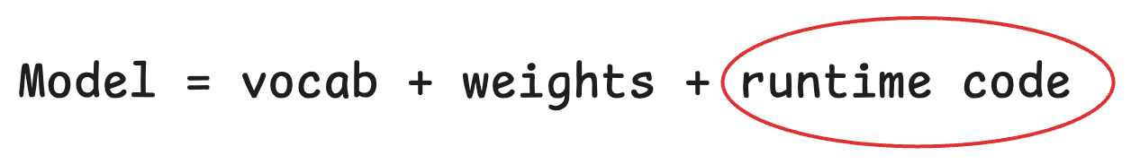
"모델"을 이야기할 때 우리는 흔히 수십억 개의 매개변수로 이루어진 거대한 파일, 즉 가중치(weights)를 떠올립니다. 하지만, 실제로 모델을 추론하기 위해서는 3가지 구성 요소를 필요로 합니다.

When we talk about "a model," we often think of the weights, those massive files measured in billions of parameters. But a model that can actually run inference requires three components:

어휘집(Vocabulary): 어휘집은 '토큰'과 '토큰 ID' 간의 정적인 매핑(Static Mapping)입니다. 즉, 사람이 읽을 수 있는 텍스트와 모델이 실제로 처리하는 숫자로 된 표현(Numerical Representation)들 간의 변환을 가능하게 하는 전체 목록입니다.

Vocabulary: A static mapping between tokens and their IDs. This is how the model translates between human-readable text and the numerical representations it actually processes.
가중치(Weights): 가중치는 학습된 매개변수, 또는 학습 과정에서 축적된 "지식"입니다. 7B 모델에는 이러한 매개변수가 70억개 있습니다.

Weights: The learned parameters, or the "knowledge" accumulated during training. A 7B model has 7 billion of these parameters.
런타임 코드(Runtime Code): 런타임 코드는 가중치를 활용하여 입력을 출력으로 변환(transform)하는 방법을 정의하는 로직입니다. GPU에서 실제로 실행되는 부분입니다.

Runtime Code: The logic that defines how to use the weights to transform inputs into outputs. This is the part that actually executes on GPUs.

추론 엔진이 모델 코드를 직접 구현하는 이유 / Why Inference Engines Implement Model Code

모델 제공자가 가중치를 공개한다면, 런타임 코드도 함께 공개하면 되지 않을까 하는 의문이 생길 수 있습니다. 실제로 많은 제공자가 그렇게 합니다. 그러나 여기에는 함정이 있습니다. 런타임 코드는 특정 시나리오에 맞게 최적화되어야 합니다. 학습 vs. 추론, 다양한 GPU 아키텍처, 다양한 정밀도 형식에 따라 다릅니다. A100 클러스터에서의 학습에 최적화된 코드가 소비자용 GPU 한 장에서 추론할 때에는 최적이 아닐 수 있습니다.

You might wonder: if model providers release weights, why don't they also release the runtime code? Many do, but there's a catch. Runtime code must be optimized for specific scenarios: training vs. inference, different GPU architectures, different precision formats. What works for training on a cluster of A100s may not be optimal for inference on a single consumer GPU.

이것이 vLLM 같은 추론 엔진이 자체적으로 모델 코드를 구현하는 이유입니다. 전체 vLLM 저장소에는 Qwen, LLaMA, DeepSeek, Mistral 등 수십 가지 모델 아키텍처에 대한 최적화된 구현이 포함되어 있습니다. Nano-vLLM은 Qwen만 지원하는 방식으로 이를 단순화하지만, 패턴 자체는 범용적입니다.

This is why inference engines like vLLM implement their own model code. The full vLLM repository contains optimized implementations for dozens of model architectures, including Qwen, LLaMA, DeepSeek, Mistral, and more. Nano-vLLM simplifies this by supporting only Qwen, but the patterns are universal.

모델 파이프라인 / The Model Pipeline

이제 토큰이 모델을 통과할 때 어떤 일이 일어나는지 추적해보겠습니다.

Let's trace what happens to a token as it flows through the model.

임베딩: 토큰에서 벡터로 / Embedding: Tokens to Vectors

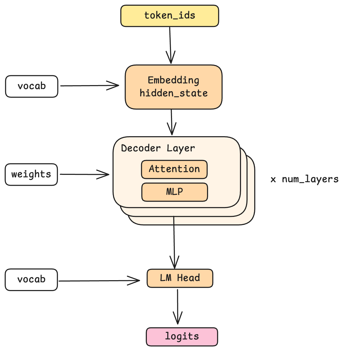
여정은 임베딩(Embedding) 에서 시작됩니다. 토큰 ID는 1547과 같은 단순한 숫자 값입니다. 임베딩 레이어는 어휘집(Vocabulary)에서 이 ID를 찾아 벡터를 가져옵니다. 이 벡터는 부동소수점의 숫자들로 이루어진 고차원 배열인데, Nano-vLLM이 사용하는 Qwen 모델에서는 4096차원입니다. 은닉 상태(Hidden State) 라고 부르는 이 벡터는 해당 토큰에 대한 모델 내부에서 사용하는 표현입니다.

The journey begins with embedding. A token ID is just a number, say, 1547. The embedding layer looks up this ID in the vocabulary and retrieves a vector: a high-dimensional array of floating-point numbers (4096 dimensions in the Qwen model Nano-vLLM uses). This vector, called a hidden state, is the model's internal representation of that token.

왜 4096차원일까요? 이는 표현력과 연산 비용 사이의 균형을 위한 설계적 선택(Design Choice)입니다. 더 고차원의 값이 되면 더 섬세한 의미를 담을 수 있지만, 그만큼 더 많은 연산과 메모리가 필요해지게 됩니다.

Why 4096 dimensions? This is a design choice that balances expressiveness against computational cost. More dimensions can capture more nuanced meanings, but require more computation and memory.

디코드 레이어: 마법이 일어나는 곳 / Decode Layers: Where the Magic Happens

은닉 상태(Hidden State)는 이후 여러 디코드 레이어(decode layers) 들을 통과합니다. Nano-vLLM이 지원하는 Qwen 모델에는 24개의 레이어가 있습니다. 각 디코드 레이어에서는 서로 다른 학습된 가중치를 사용하지만 동일한 연산을 수행하며, 이 과정에서 표현이 점진적으로 정제됩니다. 즉, 각 레이어를 통과하면서 이해의 층위가 하나씩 쌓여간다고 생각할 수 있습니다. 어떤 레이어에서는 문법적 관계를 포착하고, 다른 레이어에서는 의미론적인 뜻(Semantic Meaning)을, 또 다른 레이어에서는 사실적 지식을 처리하는 방식으로 동작할 수 있습니다. (실제로 각 레이어들이 무엇을 학습하는지는 학습 과정에서 창발적(Emergent)으로 결정되며, 명시적으로 설계되는 것이 아닙니다.)

The hidden state then passes through a stack of decode layers, 24 of them in the Qwen model that Nano-vLLM supports. Each layer performs the same operations but with different learned weights, progressively refining the representation. You can think of each layer as adding another layer of understanding: perhaps one layer captures syntactic relationships, another captures semantic meaning, another handles factual knowledge. (In reality, what each layer learns is emergent from training, not explicitly designed.)

핵심 특성은 이렇습니다. 각 레이어(Layer)에서는 은닉 상태(Hidden State)를 입력으로 받아, 은닉 상태를 출력으로 생성하며, 입력과 출력 모두 동일한 형태(4096차원)를 가집니다. 이러한 균일성이 여러 레이어를 겹겹히 쌓을 수 있게 해줍니다.

The key property: each layer takes a hidden state as input and produces a hidden state as output, both with the same shape (4096 dimensions). This uniformity is what allows layers to be stacked.

LM 헤드: 벡터에서 토큰으로 / LM Head: Vectors Back to Tokens

모든 디코드 레이어을 통과한 뒤, 최종 은닉 상태는 전체 어휘집(Vocabulary)에 대한 확률 분포로 변환됩니다. 이것이 LM 헤드(LM Head, Language Model Head) 의 역할로, 본질적으로 임베딩 과정을 반대로 수행합니다. LM 헤드의 출력값은 로짓(logits)으로, 다음에 등장할 수 있는 가능한 모든 토큰들에 대한 점수이며, 샘플링 과정을 거쳐 실제 어떠한 토큰을 선택하는지를 정하게 됩니다.

After all decode layers, the final hidden state is transformed back into a probability distribution over the vocabulary. This is the job of the LM head (language model head), which essentially reverses the embedding process. The output is logits, a score for every possible next token, which sampling then converts into an actual token selection.

디코드 레이어 내부 / Inside a Decode Layer

각 디코드 레이어은 어텐션(Attention)과 MLP라는 두 가지 주요 단계들로 구성됩니다. 하나씩 살펴보겠습니다.

Each decode layer contains two main stages: Attention and MLP. Let's examine each.

멀티-헤드 어텐션 / Multi-Head Attention

어텐션(Attention)은 각 토큰이 시퀀스 내 다른 토큰들을 "바라볼" 수 있게 하는 메커니즘입니다. 그런데 현대 LLM은 단순한 어텐션을 사용하지 않고, 멀티-헤드 어텐션(multi-head attention) 을 사용하는데, 이는 어텐션 연산을 여러개의 병렬 "헤드(Head)"로 분할합니다.

Attention is the mechanism that allows each token to "look at" other tokens in the sequence. But modern LLMs don't use simple attention. They use multi-head attention, which splits the attention computation into multiple parallel "heads."

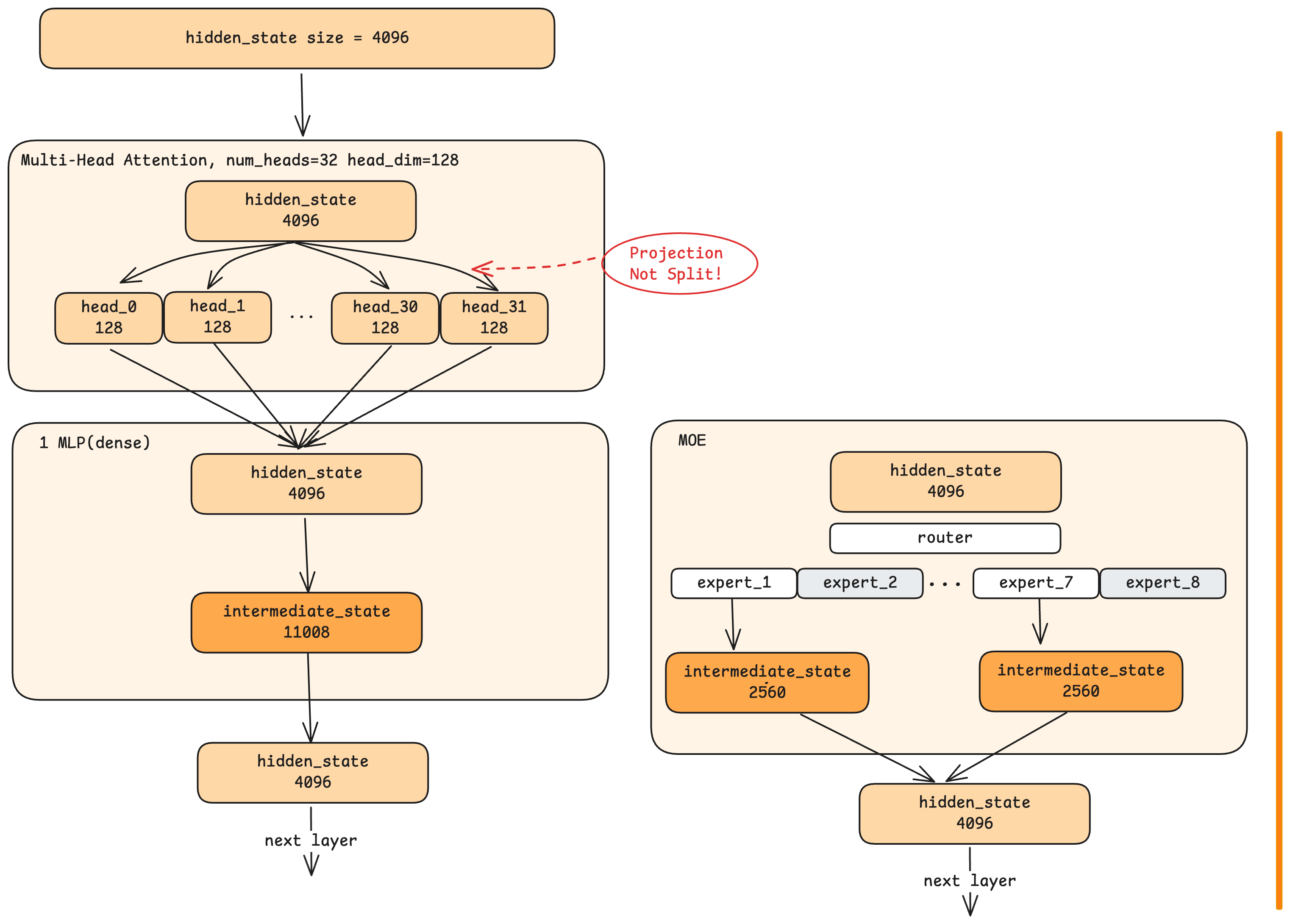
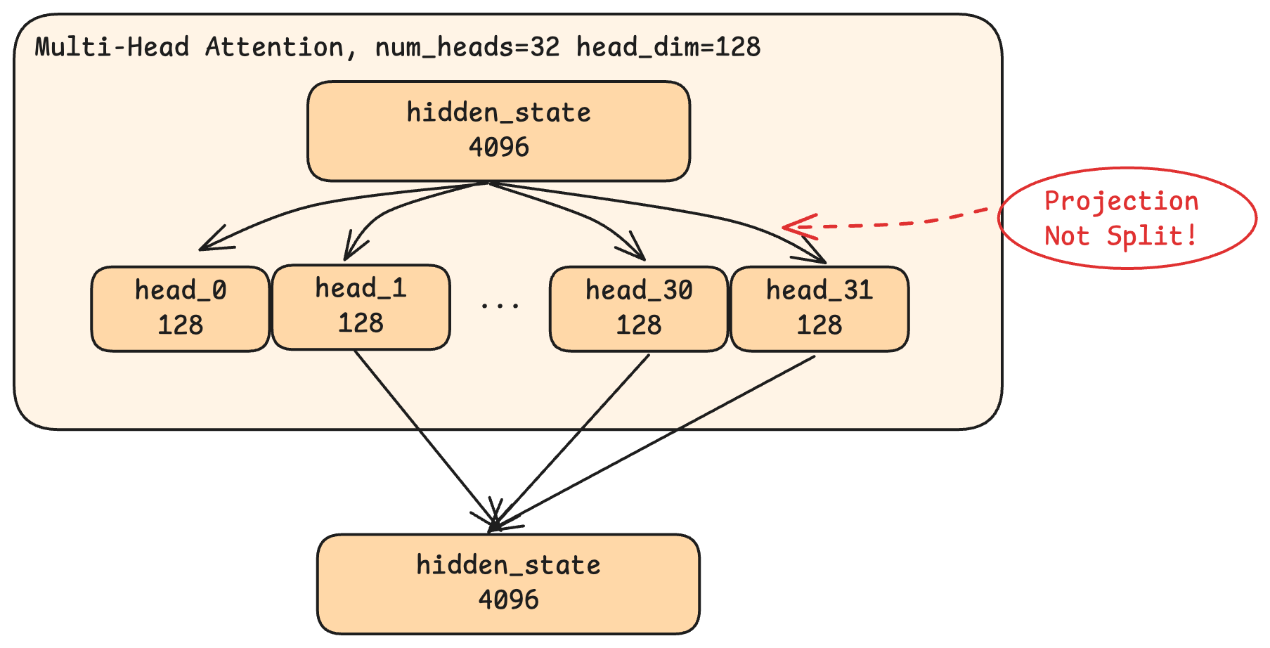
Qwen 모델에는 32개의 헤드가 있으며, 각 헤드는 전체 은닉 상태 크기(4096)를 32개로 쪼갠 128차원 분량의 데이터 조각(Slice)으로 동작(32 x 128 = 4096)합니다. 여기서 중요한 점은, 각 데이터 조각(Slice)이 단순히 입력 벡터를 순서대로 나눈 결과물이 아니라는 것입니다. 대신, 각각의 헤드는 프로젝션(projection), 즉 전체 4096차원 입력을 해당 헤드에 특화된 128차원 표현으로 압축(Compress)하는 학습된 변환(Learned Transformation)을 수행합니다.

In the Qwen model, there are 32 heads, each working with 128-dimensional slices (32 × 128 = 4096, the full hidden state size). Here's the crucial insight: this is not simply dividing the 4096 dimensions into 32 groups. Instead, each head performs a projection, a learned transformation that compresses the full 4096-dimensional input into a 128-dimensional representation specific to that head.

이를 조립 라인에 32개의 전문화된 작업대(Workstation)가 있는 공장에 비유할 수 있습니다. 각 작업대는 동일한 원자재(전체 4096차원의 입력)를 받지만, 서로 다른 도구를 사용해 특정 방식으로 가공합니다. 어떤 작업대는 문법적 적합성을 위해 깎고, 다른 작업대는 의미론적 일관성을 위해 다듬고, 또 다른 작업대는 위치적 정렬을 측정할 수 있습니다. 실제로는 각 작업대의 학습은 창발적(Emergent)으로 결정되며, 예시와 같이 딱 떨어지게 설명할 수는 없습니다.

Think of it like a factory with 32 specialized workstations on the assembly line. Each workstation receives the same raw material (the full 4096-dimensional input) but uses different tooling to shape it in a particular way. One workstation might cut for grammatical fit, another might polish for semantic coherence, another might measure positional alignment. In practice, though, what each workstation learns to do is also emergent and not so cleanly interpretable.

각 헤드는 "어텐션(Attention)" 메커니즘 자체에도 참여합니다. 각 헤드는 현재 토큰이 시퀀스의 이전 각 토큰에 얼마나 주목해야 하는지를 계산하며, 이 과정에서 모델은 문맥(Context)을 포착하게 됩니다. 즉, "The cat sat on the mat. It was comfortable."라는 문장에서 it 이 "the cat"을 가리킨다는 것을 이해하는 것입니다.

Each head also participates in the "attention" mechanism proper: it computes how much the current token should attend to each previous token in the sequence. This is where the model captures context, understanding that it in "The cat sat on the mat. It was comfortable." refers to "the cat."

모든 헤드가 연산을 완료하면, 각 헤드의 출력값들은 서로 연결(Concatenate) 된 후 다시 4096차원으로 프로젝션(Projection)됩니다. (이 과정을 통해 각 헤드가 개별적으로 파악한 정보들이 하나로 통합되며) 최종적으로 해당 레이어(Layer)의 어텐션 출력값이 생성됩니다.

After all heads complete their computations, their outputs are concatenated and projected back to 4096 dimensions, producing the layer's attention output.

MLP: 자기 정제 / MLP: Self-Refinement

MLP(Multi-Layer Perceptron) 단계는 어텐션 출력을 받아 더욱 정제합니다. 어텐션과 달리 MLP는 다른 토큰을 참조하지 않고, 각 토큰의 은닉 상태를 독립적으로 처리합니다.

The MLP (Multi-Layer Perceptron) stage takes the attention output and refines it further. Unlike attention, MLP doesn't look at other tokens. It processes each token's hidden state independently.

MLP는 먼저 은닉 상태를 4096에서 더 큰 중간 차원(Qwen에서는 11008)으로 확장(expand) 하고, 비선형 활성화 함수를 적용한 후, 다시 4096으로 압축(compress) 합니다. 이러한 확장과 압축은 왜 필요할까요?

The MLP first expands the hidden state from 4096 to a larger intermediate dimension (11008 in Qwen), applies a non-linear activation function, then compresses back to 4096. Why this expansion and compression?

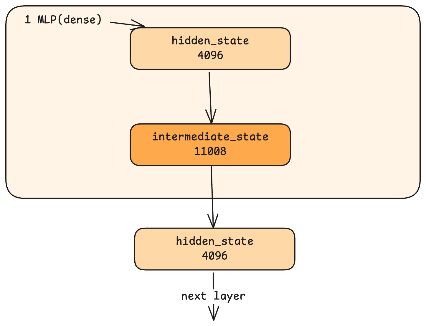
이러한 과정은 해상도를 높이는 것에 비유할 수 있습니다. 4096차원의 은닉 상태는 압축된 이미지에 비유할 수 있으며, 이를 11008차원으로 확장하는 것은 업스케일링(Upscaling)과 같습니다. MLP의 학습된 가중치를 바탕으로 세부 정보를 추가할 공간을 만드는 것입니다. 이러한 풍부한 표현을 다시 4096으로 압축하며 정제하는 과정을 거쳐, 모델은 학습 데이터에서 얻은 지식을 각 토큰의 표현에 통합합니다.

Think of it as enhancing resolution. The 4096-dimensional hidden state is like a compressed image. Expanding to 11008 dimensions is like upscaling: it creates room to add detail, informed by the MLP's learned weights. The compression back to 4096 then distills this enriched representation. Through this process, the model incorporates knowledge from its training into each token's representation.

밀집 아키텍처 vs. MoE 아키텍처 / Dense vs. MoE Architectures

지금까지 설명한 MLP는 밀집(Dense) 아키텍처입니다. 모든 토큰이 동일한 하나의 MLP 블록을 통과합니다. 하지만 일부 현대 모델들은 Mixture of Experts(MoE) 를 사용하는데, 이는 다른 접근 방식을 취합니다.

The MLP we just described is a dense architecture: every token passes through the same single MLP block. But some modern models use Mixture of Experts (MoE), which takes a different approach.

MoE에서는 하나의 큰 MLP 대신 여러 개(예를 들어 8개) 의 작은 "전문가(Expert)" MLP들이 있습니다. 여기에 라우터(router) 네트워크가 각 입력 은닉 상태를 검토하고 어떤 전문가가 처리할지를 결정합니다. 예를 들어, 8개의 전문가 중 2개만 임의의 주어진 토큰에 대해 활성화됩니다.

In MoE, instead of one large MLP, there are multiple smaller "expert" MLPs, say, 8 of them. A router network examines each incoming hidden state and decides which experts should process it. For example, only 2 out of 8 experts are activated for any given token.

"전문가"라는 용어가 사람이 해석할 수 있는 전문화를 암시할 수 있습니다. 수학 전문가, 언어 전문가, 코딩 전문가 등. 실제로 각 전문가가 학습하는 것은 학습 과정에서 창발적(Emergent)으로 결정되며, 명시적으로 설계된 것이 아닙니다. 전문가 3번이 전문가 5번과 무엇이 다른지 쉽게 설명하기는 어렵습니다.

The term "expert" might suggest human-interpretable specialization: one expert for math, another for language, another for coding. In practice, what each expert learns is emergent from training, not explicitly designed. We can't easily characterize what makes Expert 3 different from Expert 5.

그렇다면 왜 MoE를 사용할까요? 이에 대한 주된 동기는 출력 품질이 아니라 연산 효율성(Computational Efficiency) 입니다. MoE를 사용하게 되면 (모든 전문가를 합친) 전체 매개변수의 수는 많지만, 각 토큰에 대해서는 전체 매개변수의 일부만 활성화하여 토큰당 연산을 대폭 줄인 모델을 얻을 수 있습니다.

So why use MoE? The primary motivation is computational efficiency, not output quality. With MoE, you can have a model with a large total parameter count (all experts combined) while only activating a fraction of those parameters for each token. This dramatically reduces computation per token.

트레이드-오프를 살펴보겠습니다: 총 매개변수의 수가 같다고 가정할 때, 밀집 모델은 일반적으로 MoE 모델보다 더 높은 품질의 출력을 생성합니다. 밀집 모델은 모든 토큰에 대해 모든 매개변수를 사용하기 때문입니다. 하지만 매우 큰 규모에서 밀집 모델은 학습하기에 연산적으로 비현실적이 됩니다. MoE는 밀집 아키텍처로는 불가능할 규모의 매개변수 수로 확장할 수 있게 해주며, 매개변수당 효율이 다소 낮아지는 대신 실용적인 학습 가능성을 제공합니다.

The trade-off: given the same total parameter count, a dense model will generally produce higher-quality outputs than an MoE model, because the dense model uses all its parameters for every token. But dense models at very large scales become computationally prohibitive to train. MoE allows scaling to parameter counts that would be infeasible with dense architectures, accepting somewhat lower per-parameter efficiency in exchange for practical trainability.

KV 캐시: 데이터 플레인 / KV Cache: The Data Plane

이전 글(1부)에서 KV 캐시(KV Cache)의 제어 플레인(control plane) 에 해당하는 Block Manager를 살펴봤습니다. Block Manager는 CPU 메모리에서 할당을 추적하는 역할이었습니다. 이번에는 KV 캐시가 GPU 메모리에 실제로 어떻게 저장되는지, 데이터 플레인(data plane) 부분을 살펴보겠습니다.

In Part 1, we discussed the Block Manager as the control plane for KV cache, tracking allocations in CPU memory. Now let's examine the data plane: how KV cache is actually stored on GPU memory.

무엇이 캐시되는가 / What Gets Cached

어텐션 연산 중에 각 토큰은 K(key)와 V(value)의 두 개의 벡터를 생성합니다. 이 벡터들은 이후 토큰들과의 어텐션 점수(Attention Score)를 계산하는 데 사용됩니다. 매번 디코드 단계마다 이전 모든 토큰들의 K와 V를 다시 계산하는 대신, 이를 임시로 저장(Cache)해둡니다.

During attention computation, each token produces two vectors: K (key) and V (value). These are used to compute attention scores with subsequent tokens. Rather than recomputing K and V for all previous tokens at every decode step, we cache them.

물리적 레이아웃 / The Physical Layout

GPU의 KV 캐시는 다차원 구조로 구성되어 있습니다:

The KV cache on GPU is organized as a multi-dimensional structure:

블록 차원: Block Manager의 논리적 블록과 일치합니다 (예: 블록당 256개 토큰)

Block dimension: Matching the Block Manager's logical blocks (e.g., 256 tokens per block)
레이어 차원: 어텐션은 각 레이어에서 독립적으로 계산되기 때문에, 24개의 각 디코드 레이어들은 자체적으로 캐시를 가집니다.

Layer dimension: Each of the 24 decode layers has its own cache, because attention is computed independently at each layer
K/V 차원: 각 레이어 당 Key용 하나와 Value용 하나로, 총 두 개의 별도 캐시

K/V dimension: Two separate caches per layer, one for keys, one for values
토큰 차원: 각 블록 내에서, 각 토큰의 캐시된 벡터를 위한 공간

Token dimension: Within each block, space for each token's cached vectors

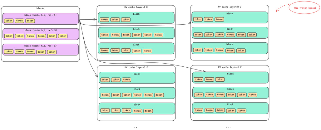
따라서 Block Manager의 단일 논리적 블록은 GPU에서 24 × 2 = 48개의 물리적 캐시 영역에 해당합니다. 24개 레이어 각각에 대해 K 캐시 하나와 V 캐시 하나씩입니다.

So a single logical block in the Block Manager corresponds to 24 × 2 = 48 physical cache regions on GPU: one K cache and one V cache for each of the 24 layers.

캐시 접근을 위한 Triton 커널 / Triton Kernels for Cache Access

Nano-vLLM은 CUDA API를 사용하여 GPU 메모리를 직접 조작하지 않습니다. 대신 효율적인 CUDA 코드로 컴파일되는 고수준 GPU 프로그램인 Triton 커널들을 사용합니다. 이 커널들이 KV 캐시의 읽기와 쓰기를 처리하며, GPU 메모리 관리의 복잡성을 추상화합니다.

Nano-vLLM doesn't manipulate GPU memory directly through CUDA APIs. Instead, it uses Triton kernels, high-level GPU programs that compile to efficient CUDA code. These kernels handle reading from and writing to the KV cache, abstracting away the complexity of GPU memory management.

텐서 병렬화: 연산 수준 / Tensor Parallelism: Computation Level

이전 글(1부)에서는 텐서 병렬화(TP)의 통신 패턴(Leader-Worker Pattern)과 리더(Leader)가 공유 메모리를 통해 명령을 전달(Broadcast)하는 방법을 알아봤습니다. 이제 실제 연산이 GPU에 걸쳐 어떻게 분산되는지 살펴보겠습니다.

In Part 1, we covered tensor parallelism's communication pattern and how the leader broadcasts commands via shared memory. Now let's see how the actual computation is split across GPUs.

어텐션에서의 병렬화 / Parallelism in Attention

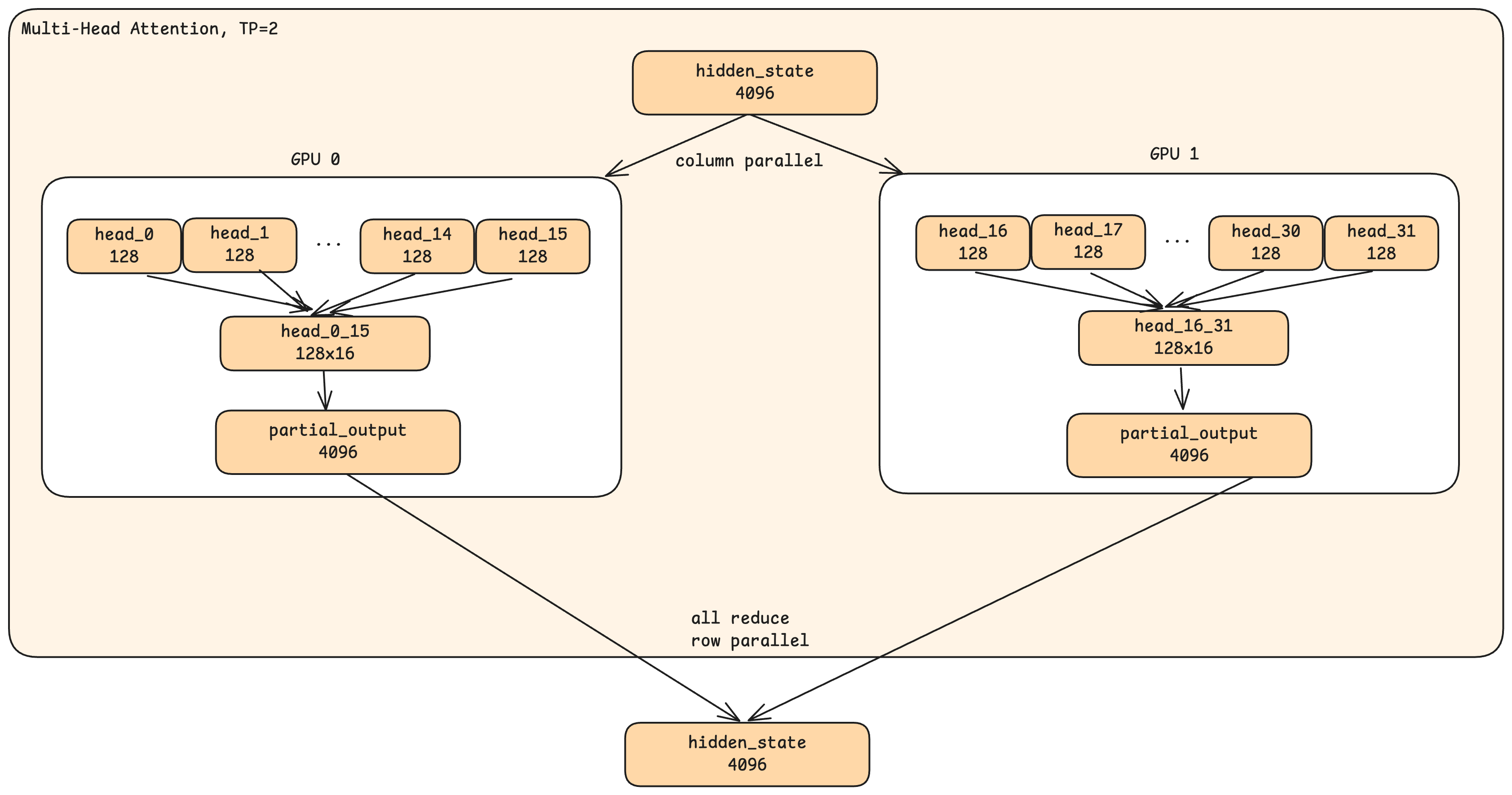
TP=2(GPU 두 개)인 상황을 가정해보겠습니다. 은닉 상태가 어텐션 단계에 들어갈 때:

Consider TP=2 (two GPUs). When a hidden state enters the attention stage:

두 GPU 모두 완전한 은닉 상태(4096차원)를 받습니다. 이 때 은닉 상태는 나뉘어지지 않고, 각 GPU가 전체 입력을 갖습니다.

Both GPUs receive the complete hidden state (4096 dimensions). This is not a split. Each GPU has the full input.
각 GPU에서 절반의 헤드(Head)를 처리합니다. GPU 0은 헤드 0~15를, GPU 1은 헤드 16~31을 처리합니다.

Each GPU handles half the heads. GPU 0 processes heads 0-15; GPU 1 processes heads 16-31.
각 GPU는 부분적인 출력을 생성합니다. GPU 0의 출력은 헤드 0~15만 반영하고, GPU 1의 출력은 헤드 16~31만 반영합니다.

Each GPU produces a partial output. GPU 0's output incorporates only heads 0-15; GPU 1's output incorporates only heads 16-31.
All-reduce가 결과를 결합합니다. GPU들이 부분 출력을 교환하고 합산하여, 둘 다 완전한 어텐션 출력을 갖게 됩니다.

All-reduce combines the results. The GPUs exchange their partial outputs and sum them, so both end up with the complete attention output.

핵심 통찰: 병렬 처리는 은닉 상태 차원이 아니라 헤드 차원에서 일어납니다. 각 GPU는 전체 입력을 보지만, 자신이 담당한 헤드만 계산합니다.

The key insight: parallelism happens in the head dimension, not the hidden state dimension. Each GPU sees the full input but computes only its assigned heads.

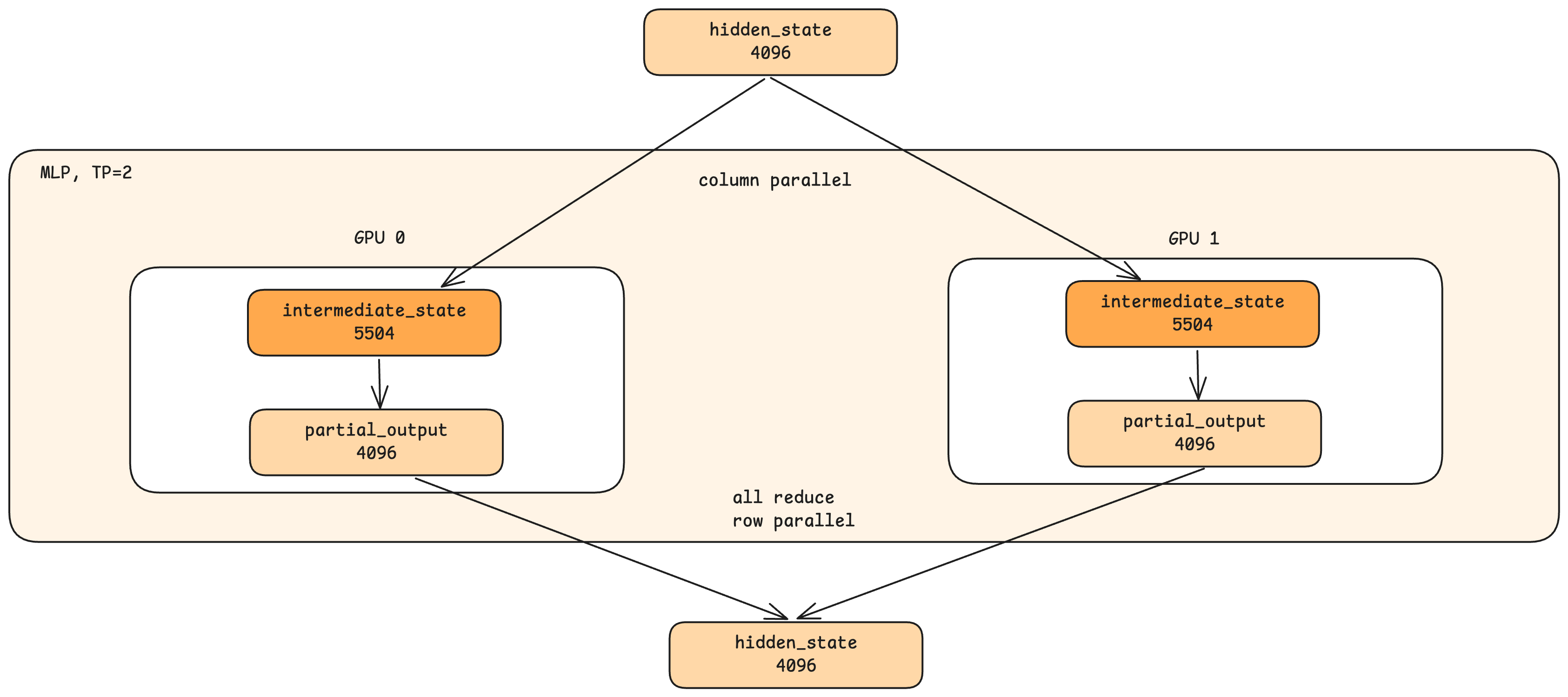
MLP에서의 병렬화 / Parallelism in MLP

MLP 병렬화도 유사한 패턴을 따릅니다:

MLP parallelism follows a similar pattern:

두 GPU 모두 완전한 은닉 상태를 받습니다.

Both GPUs receive the complete hidden state.
중간 차원이 분할됩니다. 전체 MLP가 11008차원으로 확장된다면, 각 GPU에서는 5504차원을 계산합니다.

The intermediate dimension is split. If the full MLP expands to 11008 dimensions, each GPU computes 5504 dimensions.
각 GPU에서 부분 출력을 생성합니다.

Each GPU produces a partial output.
All-reduce가 결과를 결합합니다.

All-reduce combines the results.

통신 비용 / The Cost of Communication

텐서 병렬화(TP, Tensor Parallelism)는 무료가 아닙니다. All-reduce 연산은 GPU 간 통신을 필요로 하며, 이는 지연 시간을 추가합니다. 이 때문에 TP는 통신 지연 시간이 지배하는 네트워크로 연결된 머신 간이 아니라, NVLink 등과 같이 빠른 상호 연결(Interconnect)를 갖춘 단일 머신의 여러 GPU 환경에서 가장 효과적입니다.

Tensor parallelism isn't free. The all-reduce operations require GPU-to-GPU communication, which adds latency. This is why TP is most effective on single-machine multi-GPU setups with fast interconnects (like NVLink), rather than across network-connected machines where communication latency would dominate.

그 이점은 이렇습니다. 각 GPU가 모델 가중치의 일부만 저장하면 됩니다(TP=2에서는 절반만, TP=8에서는 1/8만). 이를 통해 단일 GPU 메모리에 올라가지 않는 모델도 실행할 수 있습니다.

The benefit: each GPU needs to store only a fraction of the model weights (half for TP=2, one-eighth for TP=8). This allows running models that wouldn't fit on a single GPU's memory.

설계 트레이드-오프에 대한 고찰 / Reflections: Design Trade-offs

지금까지 내부 구조를 살펴봤으니, 자주 제기되는 몇 가지 설계 관련 질문들을 생각해보겠습니다.

Having seen the internals, let's consider some design questions that often arise.

레이어과 헤드가 제어하는 것 / What Do Layers and Heads Control?

레이어가 많을수록 일반적으로 더 깊은 추론이 가능합니다. 각 레이어가 은닉 상태에 대한 정제 과정을 한 번 더 추가하기 때문입니다. 헤드가 많을수록 더 풍부한 어텐션 패턴이 가능하며, 토큰 간의 관계를 이해하는 더 많은 "관점(Perspective)"들을 제공합니다.

More layers generally enable deeper reasoning. Each layer adds another pass of refinement over the hidden state. More heads enable richer attention patterns, giving more "perspectives" for understanding token relationships.

전문화된 깊은 추론을 위해 헤드는 적고 레이어는 많은 "좁고 깊은" 모델을 만들 수 있을까요? 또는 광범위한 지식을 위해 헤드는 많고 레이어는 적은 "넓고 얕은" 모델을 만들 수 있을까요? 연구에 따르면 이러한 구조는 잘 동작하지 않습니다. 인간의 학습과 마찬가지로, 모델도 폭과 깊이의 균형에서 이점을 얻는 것으로 보입니다. 극단적으로 불균형한 아키텍처는 성능이 저하되는 경향이 있습니다. 성공적인 모델의 대부분은 이 두 차원 사이에서 대략 정사각형에 가까운 비율을 유지합니다.

Can we create a narrow-but-deep model (few heads, many layers) for specialized deep reasoning? Or a wide-but-shallow model (many heads, few layers) for broad knowledge? Research suggests this doesn't work well. Like human learning, models seem to benefit from a balance of breadth and depth. Extremely unbalanced architectures tend to underperform. Most successful models maintain a roughly square-ish ratio between these dimensions.

모델 능력의 실질적인 키(Lever)는 학습 데이터(어떤 지식이 가용한가) 및 학습 방법론(그 지식이 얼마나 효과적으로 학습되는가)에 있으며, 아키텍처적 극단에 있지 않습니다.

The practical levers for model capability remain the training data (what knowledge is available) and training methodology (how effectively that knowledge is learned), rather than architectural extremes.

왜 MoE가 인기를 얻고 있는가 / Why Is MoE Becoming Popular?

MoE의 부상은 매개변수 당 더 나은 출력을 생성하기 때문이 아닙니다. 70B 밀집 모델(Dense Model)은 일반적으로 70B MoE 모델(70B는 모든 전문가를 합한 총합)의 성능을 능가합니다.

MoE's rise isn't because it produces better outputs per parameter. It doesn't. A 70B dense model will generally outperform a 70B MoE model (where 70B is the total across all experts).

MoE가 인기 있는 이유는 규모 확장(Scale) 이 가능하기 때문입니다. 600B 밀집 모델을 학습하는 것은 현재 인프라로는 연산적으로 비현실적입니다. 그러나 토큰당 50B 매개변수만 활성화하는 600B MoE 모델은 학습 가능합니다. 그리고 MoE 모델은 매개변수 당 효율 손실에도 불구하고, 순전한 규모로 인해 학습 가능한 어떠한 밀집 모델도 달성할 수 없는 능력을 얻을 수 있습니다.

MoE is popular because it enables scale. Training a 600B dense model is computationally prohibitive with current infrastructure. But a 600B MoE model that activates only 50B parameters per token? That's trainable. And despite the per-parameter efficiency loss, the sheer scale can achieve capabilities that no trainable dense model could match.

이는 실용적인 엔지니어링 트레이드-오프입니다: 다른 방식으로는 불가능한 규모에 도달하기 위해 매개변수 당 낮은 효율을 감수하는 것입니다.

This is a pragmatic engineering trade-off: accept lower efficiency per parameter in exchange for reaching scales that would otherwise be impossible.

결론 / Conclusion

지금까지 프롬프트에서 텍스트 생성까지의 여정을 완전히 추적해봤습니다:

We've now traced the complete journey from prompt to generated text:

토큰화(Tokenization) 는 텍스트를 토큰 ID로 변환합니다

Tokenization converts text to token IDs
임베딩(Embedding) 은 토큰 ID를 은닉 상태 벡터로 변환합니다

Embedding converts token IDs to hidden state vectors
디코드 레이어(Decode layers) 는 어텐션(토큰 간 이해)과 MLP(지식 통합)를 통해 은닉 상태를 정제합니다

Decode layers refine hidden states through attention (cross-token understanding) and MLP (knowledge integration)
KV cache는 중간 어텐션 결과를 저장해 중복 연산을 방지합니다

KV cache stores intermediate attention results to avoid redundant computation
LM 헤드(LM head) 는 최종 은닉 상태를 토큰 확률로 변환합니다

LM head converts final hidden states to token probabilities
샘플링(Sampling) 은 확률 분포에서 출력 토큰을 선택합니다

Sampling selects output tokens from probability distributions
텐서 병렬화(Tensor parallelism) 는 이 모든 것을 여러 GPU에 걸쳐 확장할 수 있게 합니다

Tensor parallelism enables all of this to scale across multiple GPUs

추론 엔진은 이러한 전체 파이프라인을 조율(Orchestrate)합니다. 요청 스케줄링부터 메모리 관리, 병렬 실행 조율까지, 모델 아키텍처는 각 단계 내의 연산을 정의합니다.

The inference engine orchestrates this entire pipeline, from scheduling requests to managing memory to coordinating parallel execution, while the model architecture defines the computation within each step.

이러한 내부 구조를 이해하면 마법처럼 보이는 것의 베일을 벗길 수 있습니다. LLM은 본질적으로 정교한 함수입니다. 벡터가 입력되고, 벡터가 출력됩니다. 지능은 매개변수의 규모, 학습 데이터의 품질, 그리고 이 모든 것을 효율적으로 실행하게 만드는 영리한 엔지니어링으로부터 발생(Emerge)합니다.

Understanding these internals demystifies what can seem like magic. An LLM is, at its core, a sophisticated function: vectors in, vectors out. The intelligence emerges from the scale of parameters, the quality of training data, and the clever engineering that makes it all run efficiently.

모델을 프로덕션에 배포하든, 성능 문제를 디버깅하든, 또는 단순히 이 시스템이 어떻게 작동하는지 궁금하든, 지금까지 살펴본 기초적인 내용이 여러분들에게 도움이 될 것입니다.

Whether you're deploying models in production, debugging performance issues, or simply curious about how these systems work, this foundation should serve you well.

이 글은 GPT 모델로 정리한 글을 바탕으로 한 것으로, 원문의 내용 또는 의도와 다르게 정리된 내용이 있을 수 있습니다. 관심있는 내용이시라면 원문도 함께 참고해주세요! 읽으시면서 어색하거나 잘못된 내용을 발견하시면 덧글로 알려주시기를 부탁드립니다.

파이토치 한국 사용자 모임이 정리한 이 글이 유용하셨나요? 회원으로 가입하시면 주요 글들을 이메일로 보내드립니다! (기본은 Weekly지만 Daily로 변경도 가능합니다.)

아래쪽에 좋아요를 눌러주시면 새로운 소식들을 정리하고 공유하는데 힘이 됩니다~